Introduction to Package

import os
from os import path
from time import time

import numpy as np

from astropy import units as u
from astropy import constants as const

%matplotlib inline
import matplotlib.pyplot as plt
import matplotlib.patches as patches
plt.rcParams['figure.figsize'] = [6, 6]
plt.rcParams['image.origin'] = 'lower'
plt.rcParams['font.size'] = 12

import peytonites
from peytonites import (
    Distribution, SimState,
    kpc_to_cm, cm_to_kpc,
    lyr_to_cm, cm_to_lyr,
    au_to_cm, cm_to_au
)

Intro

Welcome, this document is more of a quick guide, so it will be very short or in bullet points style. CGS (centimeters, grams, seconds) units are heavily favored by astronomers and astrophysicists. I am very sorry on behalf of all of us :-) So all the code in this repo uses CGS units.

Inital Conditions

These two classes that are important:

• ``SimState``: This is just a class that stores info about a time-step:

  • distribution: Particle distributions stored in a Distribution object (see next main bullet).

  • nsteps: Number of timesteps to run the simulation.

  • dt: How many seconds a single time-step is.

  • soft: Softening parameter.

  • out_interval: Output and save to file every out_interval (output is saved SimState.write(filename).

  • G: Gravitational constant in CGS. Sets the units of the simulation.

• ``Distribution``: sotres the [x, y, z, vx, vy, vz, mass] of all the paricles.

Generate Inital Condition

1. Generate Distribution

There are a cuple of models defined in peytonites/dist.py. Lets start by defining a plummer model as follows:

# User inputs
N = 200 # Number of particles
total_mass = N * (1*u.M_sun).to('g').value # Total mass of system
radius = (10*u.lyr).to('cm').value # Size of the system

# Calculate dynamical time:
# Usually dynamical_time / 100 is a good timestep
dynamical_time = peytonites.dynamical_time(total_mass, radius)

# Define model (returns a `Distribution` object):
dist = peytonites.plummer(
    N=N,
    radius=radius,
    x0=0, y0=0, z0=0,
    total_mass=total_mass,
    vx0=0.0, vy0=0.0, vz0=0.0,
    max_radius=radius
)

print(dist)

Points: 200, Distribution: Plummer

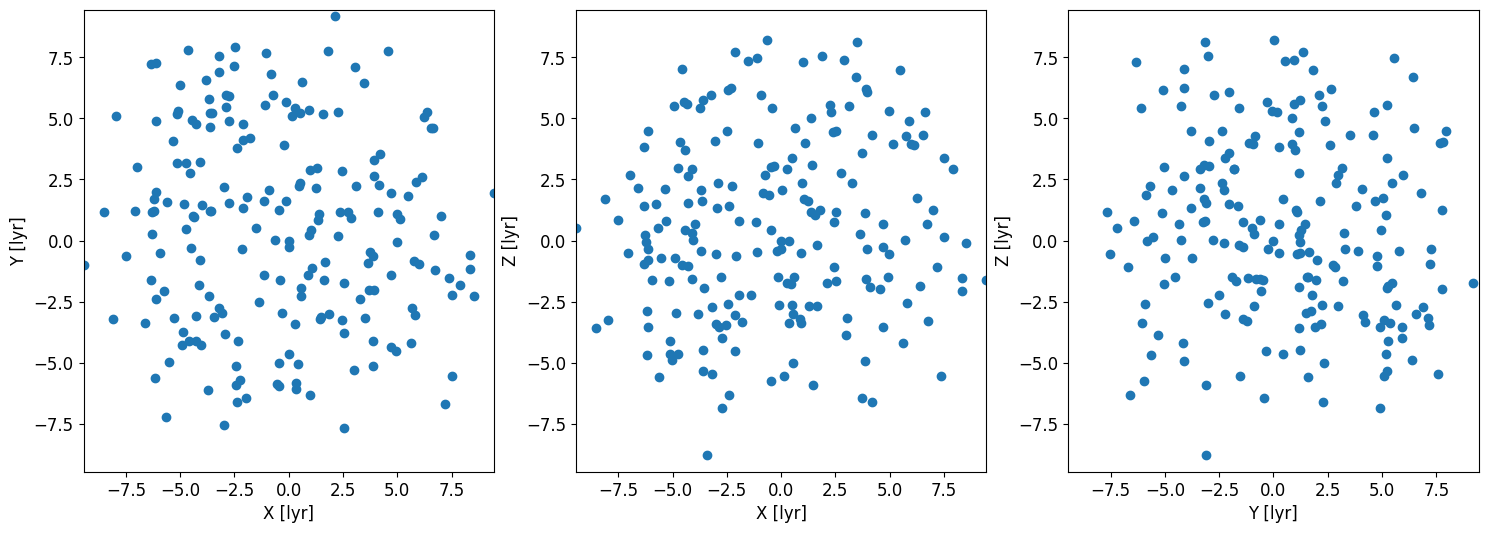
You can now access the attributes and plot as follows

# Access attributes:
some_value = dist.x * dist.y + dist.vx * dist.m

# Plot:
dist.plot(unit='lyr') # Unit is astropy unit string
plt.show()

2. Make a SimState with Simulation Params

Now we define the simulation params

# Estimate softening param based on number density and mean length:
soft = peytonites.estimate_softening_length(N, radius, fraction=0.5)

sim_init_cond = SimState(
    distribution=dist, # `Distribution` object
    nsteps=1000, # Number of steps in the sim
    dt=dynamical_time / 100, # Time interval for each time-step
    soft=soft, # Softening parameter
    out_interval=10 # Output sim every out_interval
)

You can now use this for your simulation!

Save Inital Condition

sim_init_cond.write('data/plummer_init.dat')

Load Inital Condition

sim_init_cond_from_file = SimState.read('data/plummer_init.dat')

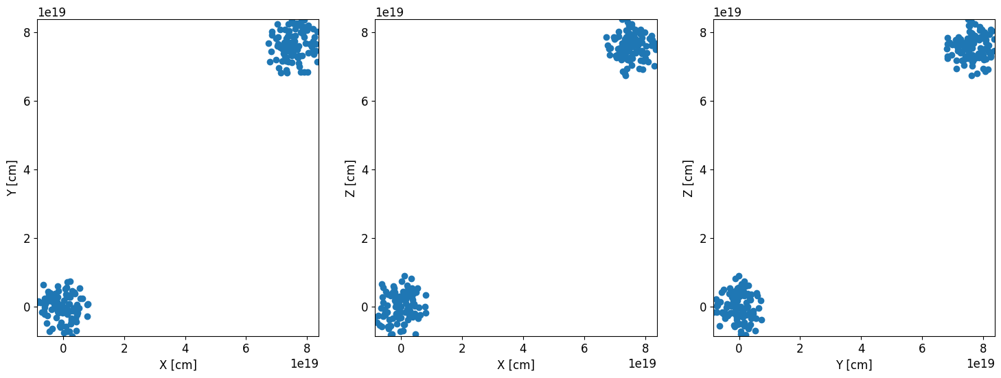
Combine Distributions

Just sum Distribution objects to combine dists

N = 200
total_mass = N * (1*u.M_sun).to('g').value
radius = (10*u.lyr).to('cm').value
dynamical_time = peytonites.dynamical_time(total_mass, radius)

dist_1 = peytonites.plummer(
    N // 2, radius,
    x0=0, y0=0, z0=0,
    total_mass=total_mass,
    vx0=0.0, vy0=0.0, vz0=0.0,
    max_radius=radius
)

dist_2 = peytonites.plummer(
    N // 2, radius,
    x0=radius*8, y0=radius*8, z0=radius*8,
    total_mass=total_mass,
    vx0=0.0, vy0=0.0, vz0=0.0,
    max_radius=radius
)


dist_combo = dist_1 + dist_2

print(dist_1)
print(dist_2)
print(dist_combo)

dist_combo.plot()
plt.show()

Points: 100, Distribution: Plummer
Points: 100, Distribution: Plummer
Points: 200, Distribution: Plummer+Plummer

Custom Distributions

To make a custom dist, just feed the Distributions class a set of points as follows:

# points is a list of particles with each particle
# being a list with the following:

points = [
    [x, y, z, vx, vy, vz, mass],
    [x, y, z, vx, vy, vz, mass],
    .
    .
    .
    [x, y, z, vx, vy, vz, mass]
]

For example:

def custom_system(N): # Params are optional
    """In CGS Units"""
    points = []
    for i in range(N):
        points.append([0, 0, 0, 0, 0, 0, 1])
    return Distribution(points, name='custom_system')

# or

def custom_system(N): # Params are optional
    """In CGS Units"""
    points = []
    x_arr = np.random.rand(N)
    y_arr = np.random.rand(N)
    z_arr = np.random.rand(N)
    vx_arr, vy_arr, vz_arr = x_arr, y_arr, z_arr
    masses = np.ones_like(x_arr)

    return Distribution.from_arrays(
        x_arr, y_arr, z_arr,
        vx_arr, vy_arr, vz_arr,
        masses, name='custom_system')

Simulation Template

def simulation(sim_init_cond, out_dir, verbose=True):

    # This part you need
    G = sim_init_cond.G # cm^3 / (g s^2)
    dt = sim_init_cond.dt
    nsteps = sim_init_cond.nsteps
    out_interval = sim_init_cond.out_interval
    soft = sim_init_cond.soft

    init_dist = sim_init_cond.distribution

    number_particles = init_dist.N

    x_arr = init_dist.x.copy()
    y_arr = init_dist.y.copy()
    z_arr = init_dist.z.copy()

    vx_arr = init_dist.vx.copy()
    vy_arr = init_dist.vy.copy()
    vz_arr = init_dist.vz.copy()

    mass_arr = init_dist.m.copy()
    for step in range(nsteps):

        #----------------#
        #                #
        # YOUR CODE HERE #
        #                #
        #----------------#

        # Output code every out_interval:
        if step % out_interval == 0:
            if verbose:
                print(step)
            step_params = sim_init_cond.copy()
            if step > 0:
                step_dist = Distribution.from_arrays(
                    x_arr, y_arr, z_arr,
                    vx_arr, vy_arr, vz_arr,
                    mass_arr, name=init_dist.name)

                step_params = sim_init_cond.copy()
                step_params.distribution = step_dist

            step_filename = 'step_{:08d}.dat'.format(step)
            step_path = path.join(out_dir, step_filename)
            if not os.path.isdir(out_dir):
                os.makedirs(out_dir)
            step_params.write(step_path)

    if verbose:
        print(step)
    return

Output Dir

Make sure to have a ``simout`` in the name for git ignore

out_dir = './plummer_simout'

Run and Time Simulation

tstart = time()
simulation(sim_init_cond, out_dir, verbose=False)
tend = time()

simulation_run_time = (tend-tstart)*u.s
print('done', 'simulation_run_time:', simulation_run_time)

done simulation_run_time: 0.3047637939453125 s

Visualizing Outputs

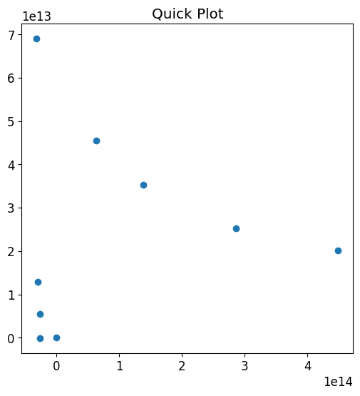
By “Hand”

out_dir = './solar_system_simout'
file_path = path.join(out_dir, 'step_00001500.dat')

# Load simulation state
step_state = SimState.read(file_path)

# Get particle distribution
dist = step_state.distribution

# Plot x and y in cm
plt.scatter(dist.x, dist.y)
plt.title('Quick Plot')
plt.show()

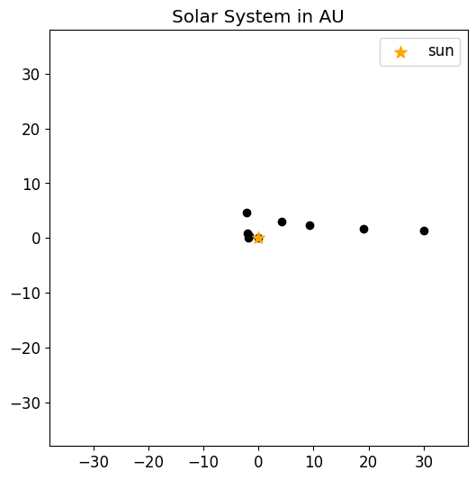
# Plot x and y in AU
# (you can also use astropy units)
plt.scatter(cm_to_au(dist.x), cm_to_au(dist.y), c='k')

# Make the sun a star
plt.scatter(cm_to_au(dist.x[0]), cm_to_au(dist.y[0]),
            marker='*', c='orange', s=100, label='sun')

plt.xlim(-38, 38)
plt.ylim(-38, 38)
plt.title('Solar System in AU')
plt.legend()

plt.show()

2D GIF

This gif will be saved in the out_dir. Its kind of slow but does the job! It will save the gif but will probably not play it here. I have added the gif below after it has been saved.

peytonites.simulation_to_gif_2d(
    out_dir,
    gif_filename='solar_sys_2d.gif',
    extent=38*u.AU,
    unit='AU'
)

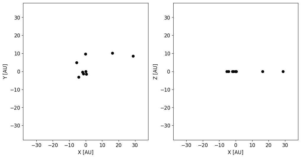
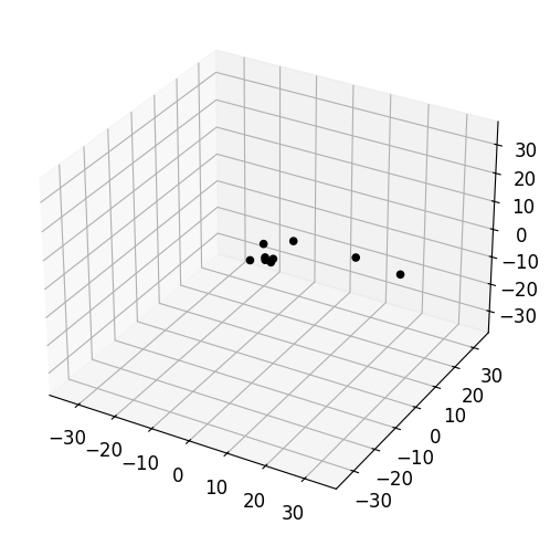
3D GIF

This gif will be saved in the out_dir. Its kind of slow but does the job!

peytonites.simulation_to_gif_3d(out_dir, gif_filename='solar_sys_3d.gif', extent=38*u.AU, unit='AU')